Art - Inspired Data Experiments on Neural Network Model Decay
Authors: Hendrik Strobelt, Mauro Martino
Introduction
While playing with the QuickDraw! data for the Forma Fluens project, we observed that taking the average of all images sharing the same label results in either a defined average image we term convergent or a blurry average image we call divergent.
The following experiments explore the properties of convergent and divergent image classes. Primarily, we test the hypothesis that convergent datasets are "easier" to learn for a neural network model than divergent datasets. We introduce a new measure called model decay to compare the robustness of generated neural networks of different depths and types. Finally, we propose several experimental measures for quantifying the divergence of a class of images and evaluate them by visual inspection.
Mixing the data
By manually reviewing the average images of the 345 labels in the QuickDraw! dataset, we select the ten most convergent labels for a convergence dataset and the ten most divergent labels for a divergence dataset.
Convergence labels (mix_00):
Divergence labels (mix_10):
To start our experiments, we create 11 different mixes of data from convergence and divergence data. Starting from the 10 convergence labels (mix_00) we iteratively remove one convergence label and replace it by a divergence label until all 10 labels are divergent (mix_10). We do this to measure a gradual drop in performance if it exists Here are some examples of datasets and how they are mixed:
80% convergence (mix_02):
70% divergence (mix_07):
We now have a series of increasingly-complex datasets for the task of multi-class classification. Click here for the dataset download link.
Experiment: (Multilayer) Perceptron
In our first experiment, we test our hypothesis by training and testing a series of twelve fully-connected neural networks of depth less than four. We find that these networks perform better on datasets with more convergent classes than on datasets with more divergent classes. We term this drop in accuracy model decay. Below are the decay curves for these networks.
Notice that these networks decay similarly over the eleven datasets. One might ask: Will some networks have a smaller decay than others? What does this mean about the robustness or suitability of those networks for classifying a dataset? Hovering over the decay curves, you may see that having more nodes in each layer leads to better performance as expected.
As an aside, let's have a look at the weights of the best performing model, the perceptron (gray line in plot above). This image represents the positive weights for a 784 x 10 net. Each column shows the weights learned for each dataset. From left to right we see the weights for the classes and how they change as we swap convergence classes for divergence classes in mix_00 to mix_10.
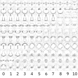
Each classes weights is influenced by all the classes. For example, note how the neck of the bottle class in the third row becomes more defined as other classes are swapped from a convergent class to a divergent class (from left to right). However, overall the changes are subtle.
Experiment: Random CNNs
The networks in the previous section are very simple and have much smaller capacity for learning complex objects in images than today's popular deep convolutional neural networks. To address this problem we create a set of 100 randomly sampled CNN architectures from a space of neural networks of depths less than 7. These networks were built from four common types of layers: convolution (blue), pooling (red), dropout (orange), and fully-connected (green). Each network was initialized using Xavier initialization and trained for 30 epochs with a learning rate of 0.001 and a batch size of 512.
These networks are visualized as columns with color-coded layer types. We test each of these networks on the 11 datasets defined above and record the decay curves pictured below. Feel free to hover around :)
We apply a linear regression to each decay curve (see below) and use the slopes as a measure of model decay.
Notice that networks with a high accuracy for the fully convergent dataset decay less than datasets with a relatively smaller accuracy. Below we show maximum accuracy vs. decay slopes. The radius of each circle indicates model depth.
and zoomed in networks with accuracy higher than 0.72:
Observation 1: We sort the model descriptions by increasing accuracy and find that the highest performing models tend to begin with a convolutional layer (blue boxes in the right side of the first row) while low performing models start with a pooling or dropout layer (red or orange boxes in the left side of the first row).
Observation 2: We think that low decay is related to higher model complexity (the number of free parameters in a neural network). For this we compare model complexity with model decay in the following plot. (The dot size indicates maximum accuracy achieved by the model).
From this plot we can read that there seems to be a tendency of robust model being more complex. Yet, complexity does not guarantee high accuracy (see e.g. small dots in upper right corner).Experiments: Quantifiable Quality
An intuitive convergence measure would be useful in quantifying the complexity of classes of spacial data such as images in solving computer vision problems.
We attempt to define a measure for convergence amongst the hundreds of quickdraw data classes that holds up to intuition. We propose and visually test three ideas.
Autoencoder Cost
First, we train and test a two-layer perceptron autoencoder as used in LeCun et al., [1] on each of the 20 classes of images and compare their respective costs using the standard L2 loss function. Although this approach seems sufficient to capture the complexity of a class, it does not match intuition as some divergent classes have lower cost than some convergent classes, which may be due to incorrect assignment of some labels as convergent instead of divergent or vice versa. It may also be due to the poor representative power of a two-layer perceptron.
Normalized Sample Variance
We notice that the average images of convergent classes show more defined edges. Thus, a measure such as pixel variance may lead to a “good” order of the classes. However, we find this to not be so since images with sharper edges and mild pixel value change across them still appear convergent.
Normalized Sample Entropy
Finally, the realization that mild pixel changes across edges can still appear convergent brings us to a measure by taking the entropy of the normalized average image. That is, we divide each average image by its maximum value and sort each 8-bit pixel value into its respective bin out of 256 possible bins. Afterwards, we find the entropy of this list as our base score. By visual inspection, this measure seems the most appropriate for the task at hand. We find near linear-separability of the convergent dataset and the divergent dataset. The entropy function scores pixel value distributions lower if they contain concentrated peaks regardless of where the peaks appear; thus, an image with pixel value peaks close to each other scores the same as peaks that are far apart. This method contains a major drawback because an image with the same pixel value at all positions will also score highly.
Further research is needed to produce an appropriate convergence measure. An additional idea is to train a convolutional neural network on a constant set of classes and an additional class to be tested. One can swap out this one class with another and retrain the model and measure model performance. However, this method has the hurdle of reconciling how the similarity of the test class with one of the base classes will affect the performance.
[1] Y. LeCun, L. Bottou, Y. Bengio, and P. Haffner. "Gradient-based learning applied to document recognition." Proceedings of the IEEE, 86(11):2278-2324, November 1998.
Download Data
We provide a download link for this dataset so that you may verify these findings and discover your own. You may download it in mnist format here. (270MB) The following convenience code will import all the datasets into a list where the first element is the full convergence dataset and the last is the full divergence dataset.
from tensorflow.examples.tutorials.mnist import input_data
DATASET_PATH = 'path/to/quickdraw_mix_dataset/'

datasets = []
for i in range(11):
    datasets.append(input_data.read_data_sets(DATASET_PATH+'conv_div_mix_%0.2i' % i))
Cite
Please use the following citation if you use the dataset for a publication.
@misc{ffdata,
	Author = {Hendrik Strobelt and Mauro Martino},
	Howpublished = {\url{https://www.formafluens.io/client/mix.html}},
	Note = {Version: 0.1},
	Title = {{Forma Fluens} model decay indicator dataset}}